


DOWNLOAD below
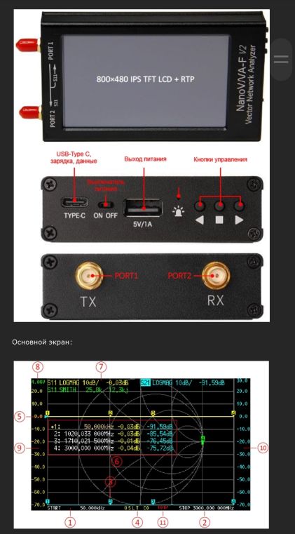
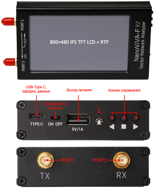
NanoVNA-F V2 is a portable vector network analyzer operating at frequencies up to 3 GHz. It is equipped with a high-quality aluminum case and a 4.3-inch IPS LCD, a built-in 5000 mAh Li-Ion battery, providing up to 7 hours of continuous operation. The screen is equipped with a touchscreen.
Note: This is a translation of the Rev. 2.0 (for firmware V0.3.0) user manual from SYSJOINT Information Technology Co., Ltd.
The design of NanoVNA-F V2 is based on edy555 NanoVNA and OwOcomm SAA-V2, the software and user interface are carefully designed and optimized. The working principle of NanoVNA-F V2 is compatible with NanoVNA-F. The measurement frequency range of NanoVNA-F V2 is expanded to 3GHz, the dynamic range is also expanded, the measurement results are more accurate, and the operation is more convenient.
Note: For unfamiliar terms and abbreviations, see the Glossary at the end of the article.
Main functions of NanoVNA-F V2:
● Dimensions: 130x75x22 mm.
● SMA RF female connectors for connecting the devices under test.
● Built-in 3.7V 5000mAh lithium battery, operating time up to 7 hours.
● Touchscreen with processing of 3 simultaneous clicks.
● Supported menu languages: English and Chinese.
● Adjustable screen brightness.
● Firmware update via virtual U disk via USB Type-C cable.
● High-quality calibration SMA attachments and RG405 cable included.
● 5V/1A USB power output port.
● Charging is carried out via USB Type-C connector, the maximum charging current reaches 2A.
● Compatible with nanovna-saver software.
● Screenshot command is supported.
Parameters of NanoVNA-F V2ParameterMeaningTerms and ConditionsFrequency range50 kHz .. 3 GHz RF output power-10dBm50 kHz .. 140 MHz-9dBm140 MHz .. 1 GHz-12dBm1 GHz .. 2 GHz-14dBm2 GHz .. 3 GHzFrequency accuracy< ±0.5ppm Dynamic range S2170dB50 kHz .. 1.5 GHz60dB1.5 GHz .. 3 GHzDynamic range S1150dB50 kHz .. 1.5 GHz40dB1.5 GHz .. 3 GHzSweep pointsmax 201Configurable within 11 .. 201Tracingmax 4 Markersmax 4 Cells for calibration settingsmax 7 Scan time1.5 sec for 101 points Screen4.3 inches IPS LCDResolution 800×480 pixelsTouchscreenRTP Built-in batteryLi 3.7V 5000mAh Data and charging portUSB Type-C Voltage for charging4.7V .. 5.5V, 2A Power outputUSB Type A, 5V/1A RF connectorsSMA mom Dimensions130x75x22 mm FrameAluminum Operating temperature range0℃ .. 45℃
Vector Network Analyzer (VNA) is a specialized instrument typically used to test antennas (impedance, reflection coefficient), RF circuits, cable losses, filter parameters, power splitters, transformers, duplexers, amplifiers, etc.
Note: Please note that “network” here does not refer to computer networks. The term “network analyzer” has existed long before computers. So here “network” refers to an electrical circuit, in this context radio frequency devices and components.
NanoVNA-F V2 has two RF ports (PORT1 TX and PORT2 RX), which can measure the S11 parameters of a circuit with one input port, or measure the S11 and S21 parameters of a circuit with two ports. If it is necessary to measure the S22 and S12 parameters of a two-port circuit, this can be done by swapping the ports with each other.
Note: Before taking measurements the VNA must be calibrated, see the “Calibration” section below.
Any quadrupole can be represented as a “black box” with a set of some parameters. There are parameter systems that connect currents and voltages at the terminals of the quadrupole, and there are also parameter systems where the quadrupole is analyzed from the point of view of incident and reflected waves (these include description via S-parameters).
S11 – reflection coefficient from the input, provided that the load at the output does not reflect energy.
S22 – reflection coefficient from the output, provided that the generator has a reflection coefficient = 0.
S21 – the coefficient of transmission of the “incident wave” from the input to the output.
S12 – on the contrary, the transfer coefficient from the output to the input.
For more details, see [4], as well as Wikipedia.
Appearance of the device and controls:
Main screen:
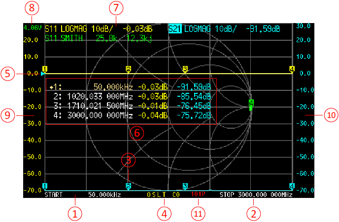
(1) Start frequency (START).
(2) Stop frequency (STOP).
(3) Marker, tracer. A marker is a pointer on a horizontal graph (tracer) displaying some characteristic (Smith chart, level, etc.). Up to 4 traces can be displayed simultaneously. The active marker can be moved along the trace to the right/left. This is done either by the side buttons UP (◄) or DOWN (►), or by touching the screen (it is recommended to use a stylus).
(4) Calibration status:
O: Indicates that OPEN calibration is in progress.
S: Indicates that SHORT calibration is in progress.
L: Indicates that LOAD calibration is in progress.
T: Indicates THROUGH (touchscreen) calibration mode.
C: Indicates that calibration has been performed for the device.
*: Indicates that calibration has been performed and applied, but has not been saved to non-volatile memory. If the power is turned off without saving, this calibration data will be lost.
c: Indicates that the calibration data is interpolated.
Cn: Indicates which calibration data has been loaded (7 data sets, n = 0 .. 6).
(5) Reference position. The reference position of the corresponding trace. The position can be changed via 【DISPLAY】 → 【REF POS】.
(6) Marker table. Up to 4 sets of markers can be displayed simultaneously, each marker is set to information including frequency and 2 other parameters. A square with the letter A at the beginning of a marker shows that it is active (you can control the marker cursor by moving it left and right). You can open, select or close a marker via the menu:
You can open, select or close a marker by:
【MARKER】 → 【SELECT】 → 【MARKER n】
To quickly activate a marker, you can click on the frequency value region of the corresponding marker line (it is recommended to use a stylus). The marker table can be moved up and down via the menu:
【MARKER】 → 【SELECT】 → 【POSITION】
The marker table can be dragged by pressing down and holding the measured value area for more than 0.5 seconds. If you want to save the marker table position setting, you can do so via the menu:
【RECALL/SAVE】 → 【SAVE】 → 【SAVE n】
(7) Trace status box. Shows the status of each trace format and the value corresponding to the active marker. For example, if the screen shows: S21 LOGMAG 10dB/ 0.03dB, it can be read as follows:
Blue tracer active
Channel: PORT2 (transmit)
Format: LOGMAG
Scale 10dB/div (scale 10 dB per division)
S21 value at current frequency 0.03dB
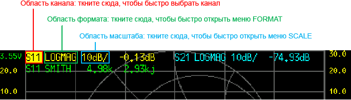
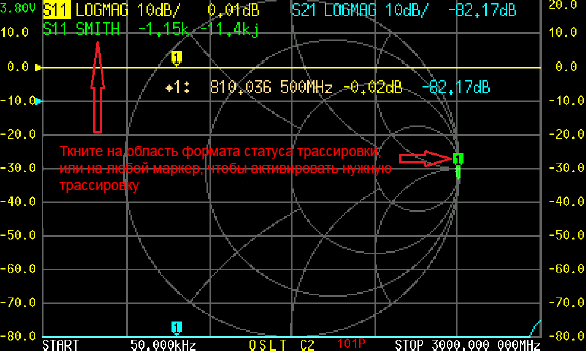
Clicking on any trace status box will activate the corresponding tracer. If the tracer is active, clicking on a specific region will trigger the shortcuts:
A tap on the “channel” region (e.g. S21) will quickly change the channel.
A tap on the “format” region (e.g. LOGMAG) will quickly open the FORMAT menu.
A tap on the “scale” region (e.g. 10dB/) will quickly open the SCALE and REFERENCE POSITION menus.
(8) Battery voltage. If the voltage is below 3.3V, please charge the device.
(9) Left ordinate. Always shows tracer mark scale 0. Tapping on the left ordinate area will quickly set the trace scale to 0.
(10) Right ordinate. Always shows the current active trace’s mark scale. Clicking on the right ordinate area will quickly set the active trace’s scale.
(11) Sweep points. Shows the configured number of sweep points (in the picture 101, can be increased to 201).
[ Main menu ]

The menu can be opened by clicking on the area shown in red in the picture above, or by pressing the middle button (■).
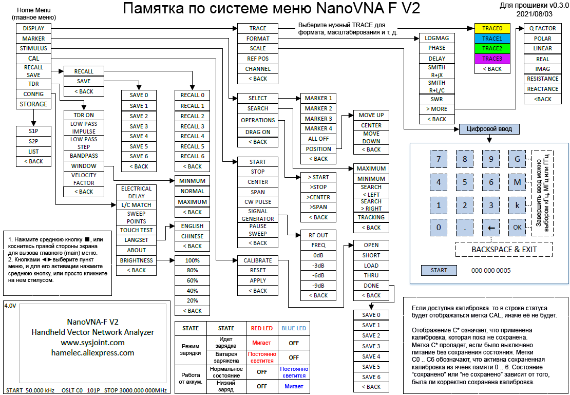

The virtual keyboard panel is used to directly enter the frequency of the scanning limits (START or STOP). It includes numeric buttons, units buttons and the ok button. The Backspace button (with the left arrow) is used to delete one character entered. When the input field is empty, clicking on the Backspace button will close the keyboard panel.
The unit selection buttons (G, M, k) select the scale of the entered number (GHz, MHz and kHz respectively).
DISPLAY . The DISPLAY menu contains 【TRACE】, 【FORMAT】, 【SCALE】, 【REF POS】, 【CHANNEL】 items:

TRACE . TRACE menu contains 【TRACE 0】, 【TRACE 1】, 【TRACE 2】, 【TRACE 3】.
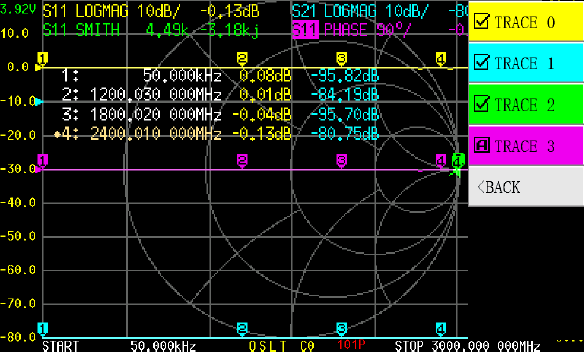
Clicking on a selected trace, such as 【TRACE 2】, will open and activate TRACE 2, and marker A will be displayed opposite TRACE 2. Clicking on another item in this menu, such as 【TRACE 3】, will open and activate TRACE 3, and marker A will now show that “TRACE 3” is active, and the marker on TRACE 2 will change to a check mark. This will open both of these tracers, and TRACE 3 will remain active.
When a tracer is active, the channel region of this tracer in the status box will be highlighted, as shown in the figure above (the purple channel S11 is highlighted). Clicking on the menu item with the marker A will close the corresponding tracer. Tracers that are marked with either a check mark or the marker A are displayed.
【FORMAT】 is used to set the format of traces. There are LOGMAG, PHASE, DELAY, SMITH R+jX, SMITH R+L/C, SWR, Q FACTOR, POLAR, LINEAR, REAL, IMAG, RESISTANCE, REACTANCE formats.
LOGMAG : The ordinate corresponds to the logarithmic amplitude, and the abscissa to the frequency.
PHASE : The ordinate corresponds to the phase, and the abscissa to the frequency.
DELAY : The ordinate corresponds to the group delay, and the abscissa to the frequency. This is only significant for channel S21.
SMITH R+jX : Shows the Smith chart impedance. The impedance is displayed in the form R+jX. This is only significant for channel S11.
SMITH R+L/C : Shows the Smith chart impedance. The impedance is displayed in the form R+L/C. where R is the active resistance component, and L/C is the equivalent inductive or capacitive reactance. This is only significant for channel S11.
SWR : The ordinate corresponds to the magnitude of the standing wave (VSWR) and the abscissa to the frequency. This is only significant for channel S11.
Q FACTOR : the ordinate corresponds to the quality factor Q, and the abscissa to the frequency.
POLAR : shows the impedance in polar coordinates. This is significant only for channel S11.
LINEAR : the ordinate corresponds to the linear amplitude, and the abscissa to the frequency.
REAL : the ordinate corresponds to the real part of the parameter S, and the abscissa to the frequency.
IMAG : the ordinate corresponds to the imaginary part, and the abscissa to the frequency.
RESISTANCE : the ordinate corresponds to the active resistance, and the abscissa to the frequency.
REACTANCE : the ordinate corresponds to the reactive component of the resistance (capacitive or inductive), and the abscissa to the frequency.
There are 3 ways to activate tracing:
– Via menu 【DISPLAY】 → 【TRACE】 → 【TRACE n】.
– By clicking on the format area of the corresponding trace in the trace status box.
– By clicking on any marker of the same color as the corresponding tracer.
SCALE . The 【SCALE】 menu is used to set the ordinate scale (not applicable to SMITH and POLAR formats).
REF POS . The 【REF POS】menu is used to set the reference position of the trace (not applicable to SMITH and POLAR formats). By default, the REF POS reference position is set to 7, which corresponds to the seventh horizontal axis from the bottom to the top (0 corresponds to the lower horizontal axis). REF POS can be set to any integer.
CHANNEL .【CHANNEL】 is used to switch the channel of the current active trace.
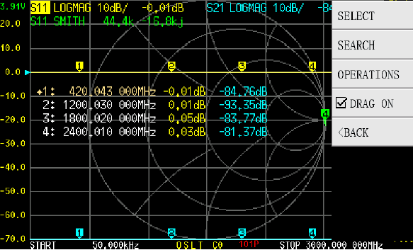
MARKER .【MARKER】menu contains【SELECT】,【SEARCH】,【OPERATIONS】,【DRAG ON】.
SELECT .【SELECT】menu contains【MARKER 1】,【MARKER 2】,【MARKER 3】,【MARKER 4】,【ALL OFF】,【POSITION】.
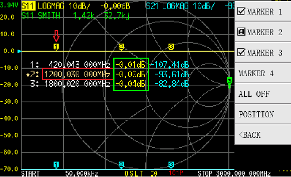
Click on 【MARKER n】(eg 【MARKER 2】) will open and activate MARKER 2, mark A will appear in front of “MARKER 2”. Click on another menu(eg 【MARKER 3】) will activate MARKER 3, and at this moment A will appear in front of “MARKER 3”, mark on “MARKER 2” will change to check mark, both MARKER 2 and MARKER 3 will remain open, and MARKER 3 will become active.
Clicking on a menu item labeled A will close the corresponding marker. The marker can only be moved with buttons when it is active.
There are 2 ways to quickly activate the marker (it is recommended to use a stylus):
– A simple poke on the marker, as shown by the red arrow in the picture above.
– A poke on the frequency value area of the corresponding marker in the marker table, as shown by the red rectangle in the picture above.
【ALL OFF】will turn off all markers at once.
【POSITION】is used to adjust the position of the marker table on the screen. The marker table can be moved up or down to avoid overlapping the traces and markers. The marker table can be moved by dragging: make sure 【DRAG ON】is enabled, then click the marker value region (as shown by the green rectangle in the figure above) and hold the click for more than 1 second, then move the marker table freely.
SEARCH . The 【SEARCH】 menu contains 【MAXIMUM】, 【MINIMUM】, 【SEARCH < LEFT】, 【SEARCH > RIGHT】, 【TRACKING】 and all functions in this menu apply to the current active marker.
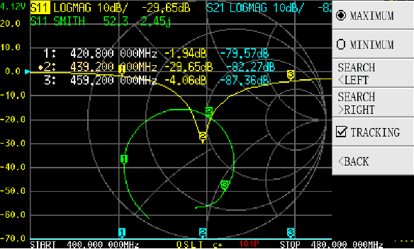
【TRACKING】is used to automatically track the maximum or minimum value of the trace. As shown in the figure above, if you want to set MARKER 2 to automatically track the minimum value of S11 LOGMAG, you must first enable MARKER 2, and then click 【MINIMUM】, and finally enable 【TRACKING】. Then MARKER 2 will automatically move to the lower point of S11 LOGMAG trace after each sweep pass.
OPERATIONS . The 【OPERATIONS】 menu contains 【>START】, 【>STOP】, 【>CENTER】, 【>SPAN】.
【>START】 will set the frequency of the current active marker to the starting frequency of scanning.
【>STOP】 will set the frequency of the current active marker to the stop scan frequency.
【>CENTER】 will set the frequency of the current active marker to the scanning center frequency.
【>SPAN】sets the frequency range between the current active marker and the next marker as the scanning range. If there is no marker near the active marker, the SPAN will be set to 0.
DRAG ON will enable/disable dragging of the marker table characteristic.
STIMULUS .【STIMULUS】menu contains【START】,【STOP】,【CENTER】,【SPAN】,【CW PULSE】,【SIGNAL GENERATOR】,【PAUSE SWEEP】.
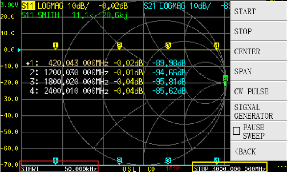
Click 【START】to set the initial scanning frequency. You can also click inside the red rectangle in the above figure to quickly set the initial frequency.
Click 【STOP】to set the stop frequency of scanning. You can also click inside the yellow rectangle in the above figure to quickly set the stop frequency.
Click 【CENTER】to set the center frequency. You can also click inside the red rectangle in the above figure to quickly set the center frequency.
Click 【SPAN】to set the scanning frequency range. You can also click inside the yellow rectangle in the above figure to quickly set SPAN.
Click 【CW PULSE】to set the CW pulse frequency. You can also click inside the red rectangle in the above figure to quickly set the CW frequency.
Please note that in this mode the PORT 1 output will be a pulsating signal, not a constantly generated frequency.
【SIGNAL GENERATOR】. NanoVNA-F V2 supports simple signal generator function, which can continuously output a specified frequency in the range of 50 kHz to 4400 MHz. The RF output power is adjustable at frequencies above 135 MHz.
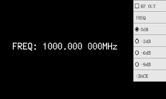
【RF OUT】Turns on/off RF output.
【FREQ】Set the frequency.
【0dB】The output power is attenuated by 0dB.
【-3dB】The output power is attenuated by 3dB.
【-6dB】The output power is attenuated by 6dB.
【-9dB】The output power is attenuated by 9dB.
PAUSE SWEEP . Click 【PAUSE SWEEP】 to pause or resume scanning.
[ Calibration ]
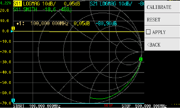
【CAL】menu contains 【CALIBRATE】, 【RESET】, 【APPLY】items.
【APPLY】is on by default, which means the calibration data has been applied. Click 【APPLY】to turn it off. After turning it off, the calibration status Cn at the bottom of the main screen will disappear, indicating that the measurement results are incorrect.
Click 【RESET】to clear the calibration data in memory. Then the OSLT Cn status at the bottom of the screen will disappear, but the calibration data saved in the internal FLASH will not be cleared. You can recall the calibration data back to memory by selecting 【RECALL/SAVE】 → 【RECALL】 → 【RECALL n】.

【CALIBRATE】 performs calibration. The following components are used for this (they are included in the device kit):
(1) SMA OPEN plug.
(2) SMA SHORT plug.
(3) SMA LOAD plug (50 ohm).
(4) SMA-JJ RG405 cable.
(5) SMA female to female adapter (optional).

To refine the calibration, you must first select the appropriate scanning frequency range (START, STOP).
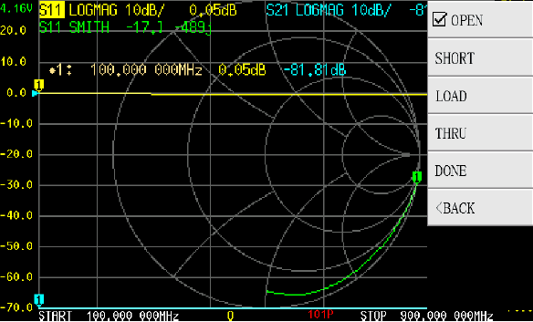
Click 【CALIBRATE】to enter the calibration interface, follow the steps below in sequence:
Step 1. At this step, the SMA OPEN plug is screwed onto PORT1. By the way, you don’t have to screw it on, because it doesn’t do anything anyway. Click on OPEN to start checking the open input. The device will beep, and after a couple of seconds, this step will be completed. A check mark will appear to the left of OPEN, and the letter “O” will appear at the bottom of the screen, indicating completion of this calibration step.
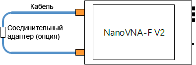
Note: DUT is usually connected to VNA by cables, which can affect the measurement, as it will be part of the measurement system. Therefore, calibration should be done through this external cable.
Step 2. Screw the SMA SHORT plug onto PORT1, click 【SHORT】, after a few seconds, the calibration at this step will be completed.
Step 3. Screw the SMA LOAD plug onto PORT1, click 【LOAD】, after a few seconds, the calibration at this step will be completed.
Step 4 : Connect PORT1 and PORT2 together with a cable, either directly or via an SMA female-to-female adapter, or via a test cable.
Click 【THROUGH】 to complete calibration.
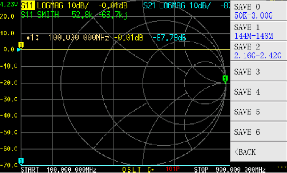
Step 5. Click 【DONE】, OSLT C* will appear at the bottom of the screen. It shows that the calibration data has been generated and applied, but not saved yet. At this time, a save menu will also appear on the right. Click 【SAVE n】to save the calibration data, after saving the calibration data, this menu item will also show the selected calibration frequency range.
After proper calibration, the VNA should have the following characteristics:
(1) When PORT1 is left open, the S11 marker of the Smith chart will be at the far right of the screen, vertically in the middle (see green marker 1 in the picture above), the S11 LOGMAG trace will be near 0dB (0.01 dB in the picture), and the S21 LOGMAG trace is best in the lowest position (-87.79 dB).
(2) When PORT1 is shorted, the S11 marker of the Smith chart will move to the left position of the pie chart, the S11 LOGMAG trace will be near 0dB, and the S21 LOGMAG trace is best in the lowest position.
(3) When PORT1 is loaded with a 50 ohm load, the S11 pointer of the Smith chart will move to the center of the screen. Small values of S11 and S21 are best.
(4) When PORT1 and PORT2 are connected to each other by cable, the S11 marker of the Smith chart should be near the center of the screen, and the S21 trace of LOGMAG should show a value of about 0dB. For the S11 trace of LOGMAG, the lower position is the best.
RECALL/SAVE . The 【RECALL/SAVE】menu contains 【RECALL】and 【SAVE】items. Click 【RECALL n】to load the previously saved calibration data from slot n. A check mark on the marker indicates that the data has been loaded. Click 【SAVE n】to save the calibration data and current settings to one of the 7 slots.
[ TDR ]
NanoVNA-F V2 can be used as a TDR reflectometer, this only works for S11.
【TDR】menu contains 【TDR ON】, 【LOW PASS IMPULSE】, 【LOW PASS STEP】, 【BANDPASS】, 【WINDOW】, 【VELOCITY FACTOR】items.
Click 【TDR ON】to enable TDR mode. Click again to disable this mode. The relationship between time domain and frequency domain is as follows.
● Increasing the maximum frequency increases the time resolution.
● A shorter measurement frequency interval (i.e. lowering the maximum frequency) increases the maximum time length.
For this reason, the maximum time length and the maximum time resolution must be in a compromise. In other words, the time length corresponds to the measured distance.
● If you want to increase the maximum measurable distance, you should reduce the number of frequency intervals (frequency span / sweep points).
● If you need to measure the distance more accurately, you need to increase the frequency range.
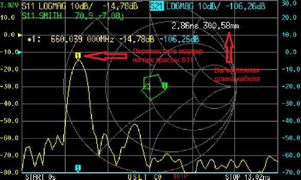
Connect the cable under test to PORT1, leaving the opposite end open or shorted. Move the marker to the peak value of trace S11, and the calculated cable length will be displayed on the screen.
There are 3 kinds of digital processing mode for TDR: 【LOW PASS IMPULSE】, 【LOW PASS STEP】, 【BANDPASS】, and the default mode 【BANDPASS】.
The range that can be measured is a finite number, and there is a minimum frequency and a maximum frequency. A window can be used to smooth out these intermittent measurement data and reduce ringing.
There are 3 levels of measurement window: 【MINIMUM】, 【NORMAL】, 【MAXIMUM】, the default is 【NORMAL】.
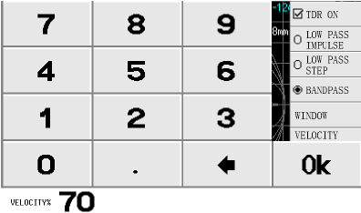
VELOCITY FACTOR . The velocity factor is defined as the ratio of the speed of propagation of electromagnetic waves along a transmission line to the speed of propagation of electromagnetic waves in a vacuum.
Click 【VELOCITY FACTOR】to set the velocity factor. For example, the typical velocity factor of RG405 cable is 0.7, for it, you should input 70 on the virtual keyboard and click Ok, then the velocity factor will be set to 70%.
Note: Use lower frequency to measure long cables and higher frequency to measure shorter cables with increased accuracy.
[ CONFIG ]
【CONFIG】menu contains 【ELECTRICAL DELAY】, 【L/C MATCH】, 【SWEEP POINTS】, 【TOUCH TEST】, 【LANGSET】, 【ABOUT】, 【BRIGHTNESS】items.
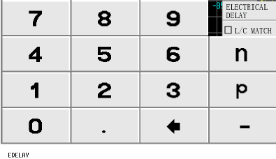
ELECTRICAL DELAY is used to set the delay time in nanoseconds (ns) or picoseconds (ps) to compensate for the delay added by connectors or cables.
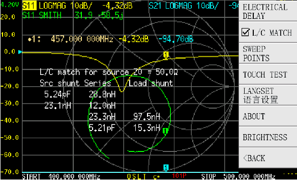
L/C MATCH . NanoVNA-F V2 supports automatic calculation of L/C matching parameters, matching the load impedance for a 50 Ohm signal source.
The structure of L/C matching circuit is shown in the figure below:

Example: the measured impedance is 31.9-58.5j, and VNA automatically generates 4 groups of suitable matching parameters:
1. 5.24pF capacitor for source shunt and 28.8nH for series inductor.
2. 23.1nH inductor for source shunt and 12nH series inductor.
3. 97.5nH inductor for load shunt and 23.3nH for series inductor.
4. 15.3nH inductor for load shunt and 5.21pF series capacitor.
SWEEP POINTS : This is the number of trace points, can be configured in the range from 11 to 201 (default is 101).
TOUCH TEST is used to check the operation of the touchscreen.
LANGSET is used to select the installed language: Chinese or English.
ABOUT . This will display the startup screen where you can see the hardware version, firmware version, serial number and support information. Each NanoVNA-F V2 has a serial number, which SYSJOINT provides after-sales service.

BRIGHTNESS . Adjusts the backlight brightness: 100%、80%、60%、40%、20%.
STORAGE . The 【STORAGE】 menu contains 【S1P】, 【S2P】, 【LIST】 items.
S1P The S11 test results can be saved to the internal memory of the NanoVNA-F V2 as S1P files, which can be exported to a PC via a USB cable.
S2P: The S11 and S21 test results can be saved to the internal memory of the NanoVNA-F V2 as S2P files, which can be exported to a PC via a USB cable.
LIST – Shows all SNP files stored on the device.
NanoVNA-F V2 supports displaying user information on the boot screen. The following installation method is used to do this:
1. Create a file callsign.txt on your PC .
2. Open the callsign.txt file in a text editor, and enter any text you want to display on the startup screen. Only ASCII characters can be entered here, for example support@sysjoint.com. The line length should not exceed 50 characters.
3. Switch NanoVNA-F V2 to flash drive mode (virtual u-disk mode), and copy the callsign.txt file to the virtual u-disk.
4. Restart NanoVNA-F V2.
[ Dictionary ]
CW Constant Wave, constant frequency, telegraph (Morse code).
DUT Device Under Test, equipment under test.
LOAD mode for 50 Ohm circuit calibration.
LOGMAG logarithmic magnitude.
RF Radio Frequency, radio frequency.
RTP Resistive Tach Panel, resistive touchscreen.
S11 , S12 , S21 parameters for evaluating radio circuits [4].
SHORT mode for short-circuited circuit calibration (zero active resistance).
SWR Standing Wave Ratio, standing wave ratio, SWR.
TDR Time Domain Reflectometry, pulse reflectometry. Allows you to find the location of damage in the cable (break or short circuit).
VNA Vector Network Analyzer, vector network analyzer.
[ Links ]
1 . Nanovna-F_V2 3G Mini vector network analyzer site:sysjoint.com.
2 . NanoVNA V2 (SAA-2) site:cqham.ru.
3 . 230219NanoVNA-F-V2.zip – firmware v0.5.0, old documentation in Russian, program Nanovna-Saver-0.3.8.
4 . S-parameters: what is it ?


You must be logged in to post a comment.